Hand-Made Vacuum Tubes

Posted by jns on November 3, 2008

The title of the film, “Fabrication d’une lampe triode” (“Build a triode vacuum tube”) may sound unusually recherché or highly metaphorical, but it is meant literally. M. Claude Paillard is an amateur radio enthusiast with an interest in historic radio equipment (or, poetically in the original: “Amoureux et respectueux des vieux et vénérables composants”). As far as I can make out from the page about this film and M. Paillard — my French is getting rusty and the Google translator is useful but not nuanced — he was involved in a project to restore an old radio station and needed to build some triode vacuum tubes.

This film illustrates how he did this from scratch. It amazes me. He demonstrates so many skills and techniques that simply are not called upon much anymore and are largely being forgotten. It all makes me feel rather dated just because I know what a vacuum tube is.

But the beauty of this film, which is almost entirely nonverbal and requires no skills in French, is that watching it will fill you in on exactly what a vacuum tube is. Okay, it won’t tell you how it works or why that’s useful in electronic circuitry, but you’ll get a remarkably tangible understanding of what’s inside, and seeing its manufacture by hand, by someone actually touching all the pieces, shaping them and putting them together to make a functional whole, is a remarkable learning experience.

Fabrication d’une lampe triode
by F2FO

More About Noise

Posted by jns on October 16, 2008

In my post about noise yesterday [at my personal blog] I added a rather inscrutable footnote about noise and power spectra. Thoughtfully, Mel asked:

I don’t quite understand this, though: “Pink noise” has a power spectrum that rolls off as the inverse of the frequency. Could you explain what that would look like, for really elementary level brains like mine?

This is just one reason why I love my Canadian friends.

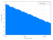
Let’s look at a couple of graphs. It doesn’t even matter that we can’t read the numbers or anything written on the graphs. We don’t have to understand them in any detail, although they’re not very complicated. We get most of what we want to understand just from the shapes of the blue parts.

    

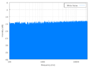
On the left is a power spectrum of white noise (Wikipedia source); on the right is a power spectrum of pink noise (Wikipedia source). Follow the links and click on the little graphs if you want to see the big versions.

The power spectrum graph plots acoustic power (loosely, how loud the component is) on the vertical axis and frequency on the horizontal axis. Frequency increases towards the right, and frequency is just what you expect: high frequencies are high pitches, low frequencies are low pitches.

If you were looking at the power spectrum of a single, pure tone (like the sounds we used to hear in the US for the emergency broadcasting system test signal, but in recent years they’ve switched to something buzzy), you would see one very narrow, tall blue spike located at the frequency of the pitch in question. If you were looking at the power spectrum of a musical instrument you would see a collection of individual, thick spikes at different frequencies that are part of that instrument’s overtone series and identify its characteristic sound.

But these are power spectra of noise, so they have components at all frequencies, which is why the graphs show solid blue regions rather than a lot of spikes–that blue region is really a huge number of blue spikes at every frequency on the graph.

It’s the shape of the top of the blue region that we want to focus on. In the spectrum on the left, the top is flat (and level), telling us that the loudness of each frequency component in the noise is equal to the loudness of every other component over the entire range we can measure.^* That’s white noise: the power spectrum is flat and every frequency component is present with equal loudness.

With pink noise, there is a shape–a specific shape–to the spectrum, as shown on the right. The top of the blue region slants downward on the right side, meaning that the loudness of any given component of the noise decreases as the frequency increases. That’s all I meant by “rolls off” really, that the curve goes down as the frequency goes up.

With the pink noise, as I said, the shape is specific. The top of the curve slants to the right but it is a flat slope^† and, for pink noise, it has a specific slope indicating that the loudness (actually the “power spectral density”, but let’s fudge it a bit and just say “loudness”) is changing exactly as the inverse of the frequency (1/f).

You can guess there’s a lot more mathematics one can delve into, but that’s more than we needed anyway. Once you see the idea of loudness vs. frequency for the graphs (“power spectra”), you can see the difference between white noise (totally flat spectrum) and pink noise (“rolls off as 1/f”).

You can hear the difference, too. Those two Wikipedia pages I linked to above have very short sound samples of synthesized white noise (approximate) and pink noise (approximate). If you listen you will notice that the white noise sounds very hissy (as I said, like TVs did in analog days when stations were off the air)–that’s because of all the relatively loud, high-frequency components. On the other hand, the pink noise sounds kind of like hearing noise under water, because the lower frequencies predominate in pink noise (water tends to filter out high frequency sounds).
———-
^*This is where practicalities come into play. Theoretical white noise would have frequency components at every possible frequency, but in practice a sound like that cannot be produced, if for no other reason than that the sound could not have gone on forever, so there are low (very, very, very low) frequency components that could not be present because there wasn’t time. Besides, audio equipment doesn’t recreate all frequencies equally, etc., and that’s why the graph of the white noise on the left isn’t exactly level but tilts up slightly towards the right side. And, of course, the top edge is fuzzy and jaggy because this is noise, and noise is random. If you were watching this on a device that measured power spectra (a spectrum analyzer–nice, but very expensive), you’d see the jagginess dance around randomly but, on average, the top would remain flat and level.

^† The graphs have logarithmic vertical and horizontal axes, with power given in decibels. However, I don’t think we need to complicate our understanding with that right now, just so long as we accept that in this kind of graph this particular straight-line slope down to the right represents the mathematical 1/f shape.

Let’s Make a Deal

Posted by jns on August 4, 2008

This is David Flannery, a lecturer in mathematics at the Cork Institute of Technology, Cork, Ireland. He is shown with his daughter Sarah Flannery, author of the book In Code : A Mathematical Journey (New York : Workman Publishers, 2001); David Flannery is listed as her coauthor.

The book is a fascinating, entertaining, and instructive one, blurbed on the jacket as “a memoir with mathematics”. It’s Sarah’s autobiographical account of her route to winning some prestigious young scientist awards in 1998 and 1999 with a good dose of mathematical fun and really good writing about the mathematical ideas at the core of public-key cryptography, if you can imagine such a thing. I enjoyed reading it very much and I think a lot of other people might enjoy it too. Here’s my book note.

Okay, so her coauthor and father happens to have a very lovely beard, but it’s all just a pretext for passing along an interesting problem and its lovely solution from an appendix of the book. I’m sure this surprises no one here.

In America this statistical brain-teaser tends to be known as the “Let’s Make a Deal” problem. Imagine you’re playing that game. Host Monty presents you with three doors: behind one is a wonderful and expensive new car, behind the other two nothing of much value. You chose one door at random. Host Monty then opens one of the two remaining doors, revealing an item of little value.

Do you change your initial choice?

Most of us who’ve done some statistics are suckered into saying “no” at first because we think that the probability of our having made the correct choice has not changed. However, it has indeed changed and a more careful analysis says we should always choose the other door after Monty opens the door of his choice. One can perhaps go along with that by realizing that Monty did not choose his door at random–he knows where the car is and he chose not to reveal the car, so the information we have at our disposal to make our “random” choice has changed.

However, seeing this clearly and calculating the attendant probabilities is neither easy nor obvious–usually. I’ve read several solutions that typically say something like “look, it’s simple, all you have to do….” and they go on to make inscrutable statements that don’t clarify anything.

The answer in Flannery’s book is the clearest thing I’ve ever read on the subject; the reasoning and calculation itself by one Erich Neuwirth is breathtaking in its transparency. From “Appendix B: Answers to Miscellaneous Questions”, this is her complete response to the question “Should you switch?”

Yes. In order to think clearly about the problem get someone to help you simulate the game show with three mugs (to act as the doors) and a matchstick (to act as the car). Close your eyes and get your helper to hide the matchstick under one of the mugs at random. Then open your eyes, choose a mug and let your helper reveal a mug with nothing under it. Play this game many times, and count how often you win by not switching and how often by switching.

The following explanation of the answer “Yes, you should switch” is from Erich Neuwirth of Bad Voeslau, Austria, and appears on page 369 of the Mathematical Association of America’s The College Mathematics Journal, vol. 30, no. 5, November 1999:

“Imagine two players, the first one always staying with the selected door and the second one always switching. Then, in each game, exactly one of them wins. Since the winning probability for the strategy “Don’t switch” is 1/3, the winning probability for the second one is 2/3, and therefore switching is the way to go.” [pp. 302--303]

Do you see the reason? Because one player always wins, the individual probabilities of each player’s winning must add up to 1. The probability of a win for the “Don’t switch” player is obviously 1/3 (1 of 3 doors chosen at random), so the probability of a win for the “Always switch” player must be 1 – 1/3 = 2/3. Brilliant!

On Satellite Dishes Looking in the Same Direction

Posted by jns on May 23, 2008

I recently finished reading Richard Dawkins’ Climbing Mount Improbable (New York : W.W.Norton & Company, 1996, 340 pages). It wasn’t bad, but it wasn’t his best by any means. All of the little things that irritate me about Dawkins’ writing seemed emphasized in this book. There’s more in my book note, of course.

Dawkins is usually such a careful writer so I was surprised by the brief lapse of analytical perspicacity he exhibits in this passage. He is describing the fascinating compass termites that build tall and surprisingly flat mounds, like thin gravestones.

They are called compass termites because their mounds are always lined up north-south–they can be used as compasses by lost travellers (as can satellite dishes, by the way: in Britain they seem all to face south). [p. 17]

Well, of course they seem to face south–the satellite dishes, I mean–and there’s a very good reason. I can’t believe Dawkins would say something this…well, I can’t think of just the right word to combine unthinking lapses with scientific naiveté, specially since he’s the Charles Simony Professor of the Public Understanding of Science at Oxford. Tsk.

Satellite dishes are reflectors for radio waves transmitted by satellites; the dishes are curved the way they are so that they focus the radio signal at the point in front of the dish where the actual receiver electronics reside, usually at the top of a tripod arrangement of struts. In order to do this effectively the satellite dish must point very precisely towards the satellite whose radio transmitter it is listening to.

If the satellite-radio dish is stationary, as most are, that means that the satellite itself appears stationary. In other words, the satellite of interest always appears at the same, unmoving point in the sky relative to the satellite dish, fixed angle up, fixed angle on the compass.

Such satellites are called “geostationary” for the obvious reason that they appear at stationary spots above the Earth. In order to appear stationary, the satellites must rotate at the same angular velocity as the Earth, and they must appear not to move in northerly or southerly directions.

In order not to appear to move north or south, and to have a stable orbit, the satellites must be positioned directly above the Earth’s equator (i.e., in the plane that passes through the Earth’s equator). In order to have the necessary angular velocity they must be at an altitude of about 35,786 km, but that detail isn’t terribly important for this purpose.

Armed with these facts, we may now consider two simple questions, the answers to which apparently eluded Mr. Dawkins:

1. For an observer in Great Britain, in what direction is the equator?
2. If a satellite dish in Great Britain wishes to listen to a geostationary satellite, in which direction will it point?

The answers: 1) south; and 2) southerly.^* Now it’s no surprise that (virtually) all satellite dishes in Britain do point south.
———-
^* Yes, there are slight complications having to do with the longitude of the particular satellite, but most of interest to Great Britain will be parked near enough to 0° longitude not to affect the general conclusion.

Edward Lorenz and His Butterflies

Posted by jns on April 30, 2008

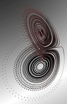The image at right is a gorgeous rendering^† of a mystifying object known as the Lorenz Attractor. It shares its name with Edward Lorenz, its discoverer, who died earlier this month at the age of 90.^* Edward Lorenz is sometimes called “the father of chaos”, and the Lorenz attractor is the reason.

Lorenz was a mathematician and meteorologist. In the early 1960s he was using what is usually described as an “extremely primitive computer” (a “Royal McBee LPG-30″) to work out some numerical solutions to a relatively simple set of equations he was using to model atmospheric convection^‡. They are a simple set of differential equations, not particularly scary, so we might as well see what they look like:

The , by the way, are not spatial variables but instead more abstract variables that represent wind velocity, pressure, and temperature in the atmosphere. You can still think of them, though, as the three dimensions of an abstract “space” that is referred to as “phase space”.^# The and are parameters in the system, numbers that get set to some value and then left at that value; parameters allow the set of equations to describe a whole family of dynamical systems.

What happened next (in the dramatic flow of time) is a story that’s been told over and over. Here’s how the American Physical Society tells it:

He [Lorenz] kept a continuous simulation running on an extremely primitive computer [!], which would produce a day’s worth of virtual weather every minute. The system was quite successful at producing data that resembled naturally occurring weather patterns: nothing ever happened the same way twice, but there was clearly an underlying order.

One day in the winter of 1961, Lorenz wanted to examine one particular sequence at greater length, but he took a shortcut. Instead of starting the whole run over, he started midway through, typing the numbers straight from the earlier printout to give the machine its initial conditions. Then he walked down the hall for a cup of coffee, and when he returned an hour later, he found an unexpected result. Instead of exactly duplicating the earlier run, the new printout showed the virtual weather diverging so rapidly from the previous pattern that, within just a few virtual “months”, all resemblance between the two had disappeared.

At first Lorenz assumed that a vacuum tube had gone bad in his computer, a Royal McBee, which was extremely slow and crude by today’s standards. Much to his surprise, there had been no malfunction. The problem lay in the numbers he had typed. Six decimal places were stored in the computer’s memory: .506127. To save space on the printout, only three appeared: .506. Lorenz had entered the shorter, rounded-off numbers assuming that the difference [of] one part in a thousand was inconsequential.

["This Month in Physics History: 'Circa January 1961: Lorenz and the Butterfly Effect' ", APS News, January 2003.]

This was a shocking result. The system of equations he was studying was nonlinear, and it is well-known that nonlinear systems can amplify small differences — Lorenz did not discover nonlinear amplification as some have written. But this divergence of the solutions was extreme: after not much time the two solutions not only weren’t close, they were so far apart that it looked like they never had anything to do with each other. This is a characteristic known as extreme sensitivity to initial conditions.

What’s more, one could put in virtually identical initial conditions all day long and keep getting different results a little ways down the road. In fact, the state of the system at these later times was unpredictable in practical terms — the system was chaotic in behavior.

That chaotic behavior was shocking result number two. Chaotic behavior had long been associated with nonlinear systems, but not with such simple systems. The behavior seemed, in essence, random, but there is no randomness at all in the equations: they are fully deterministic.^** Thus, this characteristic later became known as deterministic chaos.

Lorenz looked at the behavior of the solutions by drawing graphs of pairs of the dynamical variables as time progressed. The resulting paths are known as the system’s trajectory in phase space. The trajectory for his set of equations looped around on two different spirals, never settling down to a single line and shifting sides from one spiral to the other at unpredictable intervals. (See this image for a beautiful example that illustrates these ideas.) The image above shows how the trajectory looks, seen in quasi-3D. (Follow the strings of dots as they swoop about one loop and then fly to the other side.)

These phase-space trajectories where unlike anything seen before. Usually a trajectory would settle down into an orbit that, after some time had passed, would never change, or maybe the orbit would decay and just settle into a point where it would stay forever. Think of a coin rolling around on its side on the floor: after awhile the coin flops over and just sits on the floor in one spot forever after.

There was another oddity, too, in these phase-space trajectories Lorenz plotted. Dynamical systems that are deterministic have trajectories in phase space that never cross themselves–it’s just the way the mathematics works. However, Lorenz’ trajectories did appear to cross themselves and yet, to speak loosely, they never got tangled up. The best he could say at the time was that the planes that the trajectories were in seemed, somehow, like an infinitely thin stack of planes that kept the trajectories apart, or something.

He published his results in the March, 1963 issue of the Journal of the Atmospheric Sciences; you can download the paper online from this page, which has the abstract of the paper on it. If you look at the paper you might see that Lorenz simply didn’t have the vocabulary at the time to talk about the behavior of this system. All of that was developed about a decade later. Very few people saw his original paper and it had little impact until it was rediscovered c. 1970.

These points or orbits in phase space that are the long-time trajectories of dynamical systems are known as the attractors in the phase space, for rather obvious reasons. The Lorenz Attractor, as it became know, was an altogether stranger fish than those normal attractors. As part of the rediscovery of Lorenz’ work, in a famous and highly unreadable paper by David Ruelle and Floris Takens (“On the nature of turbulence”, Communications of Mathematical Physics 20: 167-192; 1971) the term strange attractor was created to describe such dynamical oddities of deterministic chaos as the Lorenz Attractor.^##

Strange attractors have had quite the vogue, as has deterministic chaos in dynamical systems. The characteristic feature of deterministic chaos, in addition to its unpredictability, is its extreme sensitivity to initial conditions.^&& Also in the seventies Benoit Mandelbrot’s work on fractals began to enter the mathematical-physics consciousness and the concepts developed that allowed strange attractors to be described as having non-integer dimensions in phase space. The dimension of the Lorenz Attractor is about 2.06, so it’s almost but not quite flat or, alternatively, it’s the “thick” plane that Lorenz originally conceptualized.

Lorenz has contributed to the popular culture, but few people are aware of it. His original interest was in modeling the atmosphere in the context of weather forecasting. His discovery of the Lorenz attractor and deterministic chaos (albeit not called that at the time) made it suddenly apparent that there were probably limits to how long the “long” in “long-term forecasting” could be. As he put it in the abstract to his paper, “The feasibility of very-long-range weather prediction is examined in the light of these results.” Very understated! There’s no direct calculation of the time involved–it’s probably impossible, or nearly so–but it’s generally thought that good forecasts don’t go much beyond three days. Check your own five-day forecasts for accuracy and you’ll start to see just how often things go awry around day five. The point here is that weather models are very good but there are fundamental limitations on forecasting because of the system’s extreme sensitivity to initial conditions.^††

If you’ve been reading the footnotes, you already know that Lorenz gave a paper at a AAAS meeting in 1972 titled “Does the Flap of a Butterfly’s Wings in Brazil Set Off a Tornado in Texas?” And that’s how the extreme sensitivity to initial conditions of systems exhibiting deterministic chaos became known as “the butterfly effect”.

For pretty good reasons, many people are fascinated by creating images of the Lorenz Attractor. Among other reasons it seems infinitely variable and, well, so strange. This Google images search for “Lorenz attractor” can get you started on that exploration.
———-
^† This is my source page for the image, which itself has an interesting history. It was rendered by Paul Bourke, who has a gallery featuring many beautiful images of fractals and strange attractors and related objects, of which this is just one example.

^* Some obituaries:

• Telegraph [UK]
• Wired
• New York Times

Finally, Bob Park had this to say:

EDWARD N. LORENZ: THE FATHER OF CHAOS THEORY.
A meteorologist, Lorenz died Wednesday at 90. He found that seemingly insignificant differences in initial conditions can lead to wildly divergent outcomes of complex systems far down the road. At a AAAS meeting in 1972, the title of his talk asked “Does the Flap of a Butterfly’s Wings in Brazil Set Off a Tornado in Texas.” Alas, the frequency of storms cannot be reduced by killing butterflies.

[Robert L. Park, What's New, 18 April 2008.]

^‡ The equation set is derived from the full set of equations that describe Rayleigh-Bénard convection, which is thermally driven convection in a layer of fluid heated from below. In my early graduate-school days I did some research on the topic, which may explain my early interest in chaos and related topics.

^# A “space” is quite a general thing and could be made up of any n variables and thereby be an “n-space”. However, the phrase “phase space” is generally reserved for n-spaces in which the n variables are specifically the variables found in the dynamical equations that define the dynamical system of interest. For present purposes, this footnote is entirely optional.

^** Deterministic here means pretty much what one thinks it would mean, but more specifically it means being single-valued in the time variable, or, equivalently, that the solutions of the equations reverse themselves if time is run backwards. Virtually all real dynamical systems are invariant under time reversal.

^## I tried to read part of the paper once. I remember two things about it. One was that they said the paper was divided into two sections, the first more popular in development, the second more mathematical; I couldn’t get past the first page of the first section. But I also remember how they developed some characteristics of these attractors, which seemed very peculiar at the time, and then they simply said: “We shall call such attractors ‘strange’.” Et voilà!

^&& Also expressed as exponential divergence of phase-space trajectories.

^†† The Met–the UK Meteorological Office–has an interesting series of pages about how weather forecasting works in practice, starting at “Ensemble Prediction“. The Lorenz attractor appears on the second page of that series, called “The Concept of Ensemble“.

Ceci N’est Pas Une Blog

Posted by jns on February 20, 2008

This is a blog posting about itself. According to the blog-software statistics, this is my one-thousandth posting [at my personal blog, the source for this essay] since the first one I posted on 18 October 2004.^* To be honest, I’m a bit surprised that I’m still writing here regularly three-plus years later. Evidently it works for me somehow.

I’ve noticed that one-thousand is an accepted milestone at which one is to reflect, look back, and perhaps look forward. Well, you can look back as easily as I can, and I don’t see much reason to try predicting the future since we’re going to go through it together anyway. Therefore I thought this article should be about itself.

Or, rather, the topic is things that are about themselves. So called self-referential (SR) things.

I believe that my introduction to SR things, at least as an idea, came when I read Douglas Hofstadter’s remarkable book “Gödel, Escher, Bach: An Eternal Golden Braid”. The book was published in 1979; my book of books tells me that I finished reading it on 17 August 1986, but I expect that that date is the second time that I read the book. I can remember conversations I had about the book taking place about 1980–and I didn’t start keeping my book of books until 1982.

Broadly speaking, GEB was about intelligence–possible consciousness–as an emergent property of complex systems or, in other words, about how the human brain can think about itself. Hofstadter described the book as a “metaphorical fugue” on the subject, and that’s a pretty fair description for so few words. Most of his points are made through analogy, metaphor, and allegory, and the weaving together of several themes. All in all, he took a very indirect approach to a topic that is hard to approach directly, and I thought it worked magnificently. In a rare fit of immodesty, I also thought that I was one of his few readers who would likely understand and appreciate the musical, mathematical, and artistic approaches he took to his thesis, not to mention how each was reflected in the structure of the book itself–a necessary nod to SR, I’d say, for a book that includes SR. There were parts of it that I thought didn’t work so successfully as other parts, but I find that acceptable in such an adventurous work. (The Wikipedia article on the book manages to give a sense of what went on between its covers, and mentions SR as well.)

The SR aspect comes about because Hofstadter feels that it may be central to the workings of consciousness, or at least central to one way of understanding it, which shouldn’t be too surprising since we think of consciousness as self-awareness. Bringing in SR for the sake of consciousness then explains why Kurt Gödel should get woven into the book: Gödel’s notorious “incompleteness theorems” is the great mathematical example of SR, not to mention possibly the pinnacle of modern mathematical thought.

Gödel published his results in 1931, not so long after Alfred Whitehead and Bertrand Russell published their Principia Mathematica (1910–1913). Their goal was to develop an axiomatic basis for all of number theory. They believed they had done it, but Gödel’s result proved that doing what they thought they’d done was impossible. How devastating! (More Wikipedia to the rescue: about Whitehead & Russel’s PM, and about Gödel’s Incompleteness Theorems.)

Gödel’s result says (in my words) that any sufficiently complex arithmetical system (i.e., the system of PM, which aimed to be complete) is necessarily incomplete, meaning that there are self-consistent statements of the system that can be made that are manifestly true but yet are unprovable within the system, which makes it incomplete, or that there are false statements that can be proven, which makes it inconsistent. Such statements are known as formally undecidable propositions.

This would seem to straying pretty far from SR and consciousness, but hold on. How did Gödel prove this remarkable result?^# The proof itself was the still-more remarkable result. Gödel showed how one could construct a proposition within the confines of the formal system, which is to say using the mathematical language of the arithmetical system, that said, in effect, “I am a true statement that cannot be proven”.

Pause to consider this SR proposition, and you’ll see that either 1) it is true that it cannot be proven, which makes it a true proposition of the formal system, therefore the formal system is incomplete; or 2) it can be proven, in which case the proposition is untrue and the formal system in inconsistent (contradictory). Do you feel that sinking, painted-into-the-corner feeling?

Of course, it’s the self-reference that causes the whole formal system to crumble. Suddenly the formal system is battling a paradox hemorrhage that feels rather like the Liar’s Paradox (“All Cretans are liars”) meets Russell’s own Barber Paradox (“the barber shaves all those in the town who do not shave themselves; who shaves the barber?”). When these things hit my brain it feels a little like stepping between parallel mirrors, or looking at a TV screen showing its own image taken with a TV camera: instant infinite regress and an intellectual feeling of free-fall.

Does Gödel’s Incompleteness Theorems and SR have anything to do with consciousness? Well, that’s hard to say, but that wasn’t Hofstadter’s point, really. Instead, he was using SR and the Incompleteness Theorems as metaphors for that nature of consciousness, to try to get a handle on how it is that consciousness could arise from a biologically deterministic brain, to take a reductionist viewpoint.

At about the same time I read GEB for the second time, I remember having a vivid experience of SR in action. I was reading a book, Loitering with Intent, by the extraordinary Muriel Spark (about whom more later someday). It is a novel, although at times one identifies the first-person narrative voice with the author. There came a moment about mid-way through the book when the narrator was describing having finished her book, which was in production with her publisher, how she submitted to having a publicity photograph taken for use on the back jacket of the book.

The description seemed eerier and eerier until I was forced to close the book for a moment and stare at the photograph on the back jacket. It mirrored exactly what had happened in the text, which was fiction, unless of course it wasn’t, etc. Reality and fiction vibrated against each other like blue printing on bright-orange paper. It was another creepy hall-of-mirrors moment, but also felt a moment of unrivaled verisimilitude. I think it marked the beginning of my devotion to Dame Muriel.

And that’s what this article is about. I suppose I could have used “untitled” as the title, but I’ve never figured out whether “untitled” is a title or a description. I think “undescribed” might be a still-bigger problem, though.

Now, on to the one-thousand-and-first.^%
———-
^* You’ll notice that neither the first nor the thousandth have serial numbers that correspond; the first is numbered “2″, the thousandth is numbered “1091″. Clearly I do not publish every article that I begin, evidently discarding, on average, about 9% of them. Some get started and never finished, and some seem less of a good idea when I’m finished with them than when I started.

^# And please note, this is mathematically proven, it is not a conjecture.

^% I’ve been reading stuff lately that described how arabic numerals were only adopted in the 15th century; can you imagine doing arithmetic with spelled-out numbers! Not only that, but before the invention of double-entry bookkeeping–also in the 15th century–and sometimes even after, business transactions were recorded in narrative form. Yikes!

Long Ago & Far Away

Posted by jns on February 7, 2008

In a recent comment to a post I made about reading Chet Raymo’s book Walking Zero, Bill asked an interesting question:

Jeff, there’s a question that has always bothered me. Raymo’s talk about the Hubble Space Telescope’s Ultra Deep Field image (page 174) raised it for me again. I’m sure you have the answer, or the key to the flaw in my “reasoning,” such as it is. The most distant of the thousands of galaxies seen in that image is 13 billion light years away. “The light from these most distant galaxies began its journey when the universe was only 5 percent of its present age” (174-175), and presumably only a small proportion of its present size. Now, the galaxies are speeding away from each other at some incredible speed. So if it has taken 13 billion years for light to come to us from that galaxy where it was then (in relation to the point in space that would become the earth at a considerably later date), how far away must it be now? Presumably a lot farther away than it was then?

Before we talk about the universe, I do hope you noticed that the background image I used for the “Science-Book Challenge 2008″ graphic, which you will see at right if you are reading this from the blog site (rather than an RSS feed), or which you can see at the other Science-Book Challenge 2008 page, is actually part of the Hubble Deep-Field image. If you follow the link you can read quite a bit about the project, which was run from the Space Telescope Science Institute (STScI), which is relatively nearby, in Baltimore. It’s the science institute that was established to plan and execute the science missions for the HST; flight operations are handled at Goddard, which is even closer, in Greenbelt, Maryland.

Now let’s see whether we have an answer to Bill’s question.

I think you may be able to resolve the quandary if you focus on the distance of the object seen, rather than when the light through which we see it left its bounds.

The object’s distance is the thing that we can determine with reasonable accuracy (and great precision) now, principally through measuring red shifts in spectra of the object.^* One of astronomer Hubble’s great achievements was determining that the amount of red-shift, which depends on our relative velocity, corresponds directly with the distance between us and the observed object.^# So, take a spectrum, measure the red shift of the object, and you know more-or-less exactly how far away it was when the light left it.

Oh dear, but that doesn’t really settle the issue, does it? On the other hand, it may be the most precise answer that you’re going to get.

Saying that, when the light left the object, the universe was only 5% its current size should be seen more as a manner of speaking than a precise statement. It can be a rough estimate, along these lines. Say the universe is about 14 billion years old and this object’s light is 13 billion years old, and if the universe has been expanding at a uniform rate, the the universe must have been (14-13)/14ths or about 7% its current size (which is about 5% its current size).

But I’d say you should treat that just as something that makes you say “Wow! That was a long time ago and the universe must have been a lot different”, and don’t try to extrapolate much more than that.

It’s probably true that the universe hasn’t been expanding at a uniform rate, for one thing. There’s a theory that has had some following for the past 25 years, called the theory of inflation.^** For reasons that have to do with the properties of matter at the extreme compression of the very, very early universe, the theory suggests that there was an “inflationary epoch” during which the universe expanded at a vastly faster rate than is visible currently. Now, some of the numbers involved are astonishing, so hold on to your seat.

The inflationary epoch is thought to have occurred at a time of about seconds after the big bang, and to have lasted for about seconds.^## During this time, it is thought that the universe may have expanded by a factor of . (One source points out that an original 1 centimeter, during inflation, became about 18 billion light years.)

So, inflation would rather throw a kink into the calculation, not to mention the possibility that the universe is not expanding in space, but that space itself is expanding. That can make calculations of what was where when a touch trickier.

But that’s not the only problem, of course. I can hear Bill thinking, well, that may all be so, but if we’re seeing the distant object as it was 18 billion light years ago, what’s it doing now.

I’m afraid that’s another problem that we’re not going to resolve, and not for lack of desire or know-how, but because of physical limitation. The bigger, tricker issue is — and I almost hate to say it — relativity. No doubt for ages you’ve heard people say of relativity that it imposes a universal speed limit: the speed of light. Nothing can go faster than the speed of light. That’s still true, but there’s an implication that’s not often spelled out: the breakdown of simultaneity, or what does it mean for thing to happen at the same time?

It’s not usually a tricky question. Generally speaking, things happen at the same time if you see them happen at the same time. Suppose you repeat Galileo’s famous experiment of dropping two different weights from the leaning tower of Pisa at the same time (he said he would), and you observe them hitting the ground at the same time. No real problem there: they fell right next to each other and everyone watching could see that they happened at the same time.

Suppose the objects are not next to each other though. Suppose instead that we observe some event, say, a meteor lands in your front yard. 8.3 minutes later you observe a solar flare on the sun through your telescope. “Isn’t that interesting,” you say, “since the Earth is 8.3 light-minutes from the Sun, that flare and my meteor’s landing happened at the same time.”

Well, the problem here, as you may have heard about before, is that an observer traveling past the Earth at very high speeds and using a clock to measure the time between the two events, your meteor and the solar flare, would deduce that the two events did not happen at the same time. The mathematics is not so difficult, but messy and probably not familiar. (You can see the equations at this page about Lorentz Transformations, or the page about Special Relativity.)

What happens is that in order for the speed of light to be constant in all inertial reference frames–the central tenet of special relativity–causality breaks down. Events that appear simultaneous to one observer will, in general, not appear simultaneous to another observer traveling at a uniform velocity relative to the first observer. (This cute “Visualization of Einstein’s special relativity” may help a little, or it may not.) Depending on the distance between two events, different observers may not even agree on with event happened first.

So, the not-so-satisfactory answer, Bill, is a combination of 1) because of inflation, it may not be so very much further away than it was 13 billion years ago; but 2) because of the breakdown of simultaneity due to special relativity, we can’t say what it’s doing now anyway, because there is no “now” common to us and the object 13 billion light-years away.^%

Gosh, I do hope I answered the right question!
———-
^* You may recall that red shift refers to the Doppler effect with light: when objects move away from us, the apparent wavelength of their light stretches out–increases–and longer wavelengths correspond to redder colors, so the light is said to be red-shifted. This happens across the entire electromagnetic spectrum, by the way, and not just in the visible wavelengths.

^# Applying Hubble’s Law involves use of Hubble’s Constant, which tells you how fast the expansion is occurring. The curious thing about that is that Hubble’s Constant is not constant. I enjoyed reading these two pages: about Hubble’s Law and Hubble’s Constant. The second one is rather more technical than the first, but so what.

^**Two useful discussions, the first shorter than the second: first, second.

^## Yes, if you want to see how small a fraction of a second that was, type a decimal point, then type 31 zeroes, then type a “1″.

^% I leave for the interested reader the metaphysical question of whether this statement means that universal, simultaneous “now” does not exist, or that it is merely unknowable.

When Celsius = Fahrenheit

Posted by jns on February 6, 2008

A while back, someone ended up at a page on this blog by asking Google for “the temperature at which the Celsius scale and Fahrenheit scale are the same number”. I don’t think they found the answer because I’d never actually discussed that question¹, but I thought the question was pretty interesting and discussing the answer might be a bit of good, clean rocket-science fun.

Actually, there is a prior question that I think is interesting, namely: how do we know that there is a temperature where the Celsius and Fahrenheit scales agree? The answer to that question is related to a simple mathematical idea.² We can picture this mathematical idea by drawing two lines on a chalkboard (or whiteboard) with a rule.

First, draw line A any way you want, but make it more horizontal than vertical, just to keep things clear. Now, draw line B in such a way that it’s point farthest left is below line A, but its point farthest right is above line A. What you will always find that that line B and line A will cross at some point. This may seem like an obvious conclusion but it is also a very powerful conclusion. Now, knowing where they will cross is another, often more difficult, question to answer.

How do we know, then, that the Fahrenheit and Celsius lines cross? Well, the freezing point of water, say, on the Celsius scale is 0°C, and on the Fahrenheit it is 32°F. On the other hand, absolute zero is -273.15°C, but -459.67°F. So, at the freezing point of water the Fahrenheit line is above the Celsius line, but at absolute zero that situation is reversed.

Finding the point where they cross is a simple question to answer with algebra. The equation that converts Fahrenheit degrees into Celsius degrees is

The equation that goes the other way is

To find the temperature where the two lines cross, take one of the equations and set

so that

and then solve for . The result is that

[Addendum: 19 February 2008, for the Kelvin & Fahrenheit folks]

The Kelvin scale of temperatures is a thermodynamic temperature scale: it’s zero point is the same as zero temperature in thermodynamic equations. It used Celsius-sized degrees, and there is indeed a temperature at which the Kelvin and Fahrenheit scales cross. The relation between the two is

(Note that the absolute temperature scale uses “Kelvins” as the name of the units, and not “degrees Kelvin”.) As in the Fahrenheit / Celsius example, set and solve for , with the result that

As before, Fahrenheit degrees are larger than Kelvins and will eventually overtake them, but the initial difference between the zero points is much larger, so the crossing point is at a much higher temperature.
———-
¹Because of the way links on blogs select different combinations of individual posts, by days, by months, by topics, etc., internet search engines often present the least likely links as solutions to unusual word combinations in search strings. I find this phenomenon endlessly fascinating.

²The mathematical idea is one that I’ve always thought was a “Fundamental Theorem of [some branch of mathematics]“, but I’ve forgotten which (if I ever knew) and haven’t been able to identify yet. This is probably another effect of encroaching old-age infirmity.
I imagine — possibly remember — the theorem saying something like:

For a continuous function defined on the interval , for , takes on all values between and .

Easy Entropy

Posted by jns on February 3, 2008

Thermodynamics is the theory that deals with heat and heat flow without reference to the atomic theory; it was developed at the same time as the steam engine and the family resemblances are striking. All concepts about temperature and pressure in terms of our perceptions of atomic or molecular motion came later and properly belong in the discipline known as Statistical Mechanics.

Awhile back I read this bit in the referenced book and thought it shed a lot of light on the idea of entropy, about which more after the excerpt.

Clausius saw that something was being conserved in Carnot’s [concept of a] perfectly reversible engine; it was just something other than heat. Clausius identified that quantity, and he gave it the name entropy. He found that if he defined entropy as the heat flow from a body divided by its absolute temperature, then the entropy changes in a perfectly reversible engine would indeed balance out. As heat flowed from the boiler to the steam, the boiler’s entropy was reduced. As heat flowed into the condenser coolant, the coolant’s entropy increased by the same amount.

No heat flowed as steam expanded in the cylinder or, as condensed water, it was compressed back to the boiler pressure. Therefore the entropy changed only when heat flowed to and from the condenser and the boiler and the net entropy was zero.

If the engine was perfectly reversible, it and the surroundings with which it interacted remained unchanged after each cycle of the engine. Under his definition of entropy Clausius was able to show that every thing Carnot had claimed was true, except that heat was conserved in his engine.

Once Carnot’s work had been relieved of that single limitation, Clausius could reach another important result: the efficiency of a perfectly reversible heat engine depends upon nothing other than the temperature of the boiler and the temperature of the condenser.

[John H. Lienhard, How Invention Begins (Oxford : Oxford University Press, 2006) p. 90]

Amazing conclusion #1: virtually everything about heat flowing from a warm place to a cool place depends only on the difference in temperature between the warm place and the cool place.

Amazing conclusion #2: there is an idea, call it entropy, that encapsulates #1. If we let stand for entropy, and stand for the change in entropy, then we can write

This is Clausius’ definition in symbols.

Now, there’s a lot of philosophical, interpretative baggage that travels with the idea of entropy, but if you can keep this simple approach in mind you can save a lot of heartburn pondering the deeper meaning of entropy and time’s arrow and the heat-death of the universe.

Entropy is an accounting tool. When heat flows between the hot place and the cold place, at best, if you allow it very carefully, you may be able to reverse the process but you will never do better, which means that you will never find the cold place getting colder than originally, nor the hot place getting hotter than originally, no matter what you do, unless you put still more heat into the system.

That’s one version of the notorious “Second Law of Thermodynamics”. There are a number of other forms.

For instance, another way of saying was I just said: entropy never decreases. There, thermodynamic accounting made easy.

Another one that’s useful: if you construct a device that uses heat flowing from a hot place to a cold place to do mechanical work — say, in a steam engine — some of the heat is always wasted, i.e., it goes into increasing entropy. Put another way: heat engines are never 100% efficient, not because we can’t build them but because it is physically impossible.

Think for a moment and you’ll see that the implication of this latter form of the Second Law of Thermodynamics is a statement that perpetual motion machines are impossible. They just are, not because a bunch of physicists though it might be a good idea to say it’s impossible, but because they are. That’s the way the universe is made.

Entropy needn’t be scary.
———-
^* is a general purpose symbol often used to indicate a change in the quantity represented by the letter following it.

The Pendulum Swings

Posted by jns on January 30, 2008

Sometimes I’m just reading, minding my own business, when the oddest things smack me squarely in the forehead. For instance:

As believers in faith and ritual over science, perhaps it’s not surprising that they [Evangelical Christians, as it turns out] failed to heed the basic laws of physics.

Most people understand that when a pendulum is pushed too far in one direction, it will eventually, inexorably swing back just as far to the opposite side. This is the natural order of things, and it tends to apply across the board — even to that bulwark of chaos theory, politics.

[Chez Pazienza, "Losing Their Religion", Huffington Post, 30 January 2008]

Whatever is this person talking about and where did s/he get the crazy notions about “the basic laws of physics” on display in these few sentences? (It seems about as nonsensical to me as people who use “literally” to mean “really, really metaphorically”.)

Based on the laws of physics, I believe that a pendulum is a physical object that swings back and forth, often used to keep time. I also believe that if it’s pushed far enough in one direction is will eventually break or, at the very least, enter a non-linear mode of oscillations. In my book, it is in the nature of pendula, even when swung a little in one direction, to swing in the other direction, and then back again in the original direction.

It is this oscillatory nature of the pendulum that is referred to in the metaphorical pendulum of politics and public opinion. Perhaps our author is thinking of a spring that, when squeezed, or stretched, in one direction will spring back just as far in the opposite direction?

As for politics being the bulwark of chaos theory — WTF? Someday, perhaps when we have more time, we’ll talk about some interesting history and results in chaos studies, but I don’t think politics will get mentioned, alas.

A pendulum is a fascinating thing, of course. Its use in clocks as a timing governor^* is traced to Galileo’s observation that the period of oscillation depends only on the length of the pendulum and not on the amplitude of its swing. The period (“T”) depends only on the length (“L”) of the pendulum and the acceleration due to gravity (“g”–a constant number):

Now, this is really an approximation with some assumptions like a) the pendulum has all its weight at the swinging end; and b) the amplitude of the swing isn’t too big. But it’s really a very good approximation, good enough for very precise horological instruments.

This equation tells us a couple of interesting things. One is that, because of the square-root sign over the length, if you want to double (multiply by 2) the period of a pendulum you must increase its length by 4; likewise, for half the period make the length one-fourth the original.

This also tells us that tall-case clocks tend to be much the same size. Generally speaking, they are constructed to house a pendulum with a two-second period, i.e., a pendulum that takes precisely one second to swing either way, or one second per tick, one second per tock. The length of such a pendulum is very nearly 1 meter.

At our house we also have a mantel clock that is, not surprisingly, a little under 12 inches tall because it has a pendulum with a period of 1 second, i.e., one second for a complete back-and-forth swing; such a pendulum has a length of about 0.25 meters, or one-quarter the tall-case clock’s pendulum.

Many tall-case clocks that I’ve seen have a pendulum whose rod is actually made from a flat array of a number of small rods, usually in alternating colors. This is a merely decorative vestige of the “gridiron pendulum” invented by master horologist John Harrison in 1720. The pendulum is constructed of two types of metal arranged so that the thermal expansion of one type of metal is compensated for by the thermal expansion of the other. (It’s easiest to look at an illustration, which is discussed here.)
———-
^* The pendulum, coupled with an escapement mechanism, is what allows a pendulum clock to tick off uniform intervals in time.